What is Statistics?
The field of statistics is the science of learning from data. Statistical knowledge helps you use the proper methods to collect the data, employ the correct analyses, and effectively present the results. Statistics is a crucial process behind how we make discoveries in science, make decisions based on data, and make predictions. Statistics allows you to understand a subject much more deeply.
What makes statistics important for Data Science?
Statistics is a Mathematical Science pertaining to data collection, analysis, interpretation, and presentation. Statistics is used to process complex problems in the real world so that Data Scientists and Analysts can look for meaningful trends and changes in Data. In simple words, Statistics can be used to derive meaningful insights from data by performing mathematical computations on it.
Moving ahead let’s discuss the basic terminologies in Statistics.
Basic Terminologies In Statistics :
One should be aware of a few key statistical terminologies while dealing with Statistics for Data Science. I’ve discussed these terminologies below:
Variable
A variable is an attribute that describes a person, place, thing, or idea. The value of the variable can “vary” from one entity to another.
For example, a person’s hair color is a potential variable, which could have the value of “Black” for one person and “Red” for another.
Variables can be classified as
- Qualitative (categorical)
- Quantitative (numeric)
Qualitative
Qualitative variables take on values that are names or labels. The color of a ball (e.g., red, green, blue) or the breed of a dog (e.g., collie, shepherd, terrier) would be examples of qualitative or categorical variables.
Quantitative
Quantitative variables are numeric. They represent a measurable quantity. For example, when we speak of the population of a city, we are talking about the number of people in the city a measurable attribute of the city. Therefore, the population would be a quantitative variable.
Quantitative variables can be further classified as Discrete or Continuous.
- Continuous. If a variable can take on any value between the range of minimum and maximum value, it is called a Continuous variable. Example for continuous variable: If your variable is “ The Height of the PoliceMen between 170-190 cm, which can be infinite, then the height of policemen would be an example of a Continuous variable.
- Discrete. If a variable takes discrete values which can be integers, real numbers, etc., then it is called a Discrete variable.
Example of discrete variable: If your variable is “Number of planets around a star,” then you can count all of the numbers out (there can’t be an infinite number of planets). That is a Discrete variable.
Statistical data are often classified according to the number of variables being studied.
Univariate data
When we conduct a study that looks at only one variable, we say that we are working with univariate data. Suppose, for example, that we conducted a survey to estimate the average weight of high school students. Since we are only working with one variable (weight), we would be working with univariate data.
Bivariate data
When we conduct a study that examines the relationship between two variables, we are working with bivariate data. Suppose we conducted a study to see if there were a relationship between the height and weight of high school students. Since we are working with two variables (height and weight), we would be working with bivariate data.
Levels of measurement in statistics :
The level of measurement in about how each variable is measured i.e. qualitative or quantitative and how precise each variable is
A variable has one of four different levels of measurement:
- Nominal. The nominal scale is a naming scale, where variables are simply named or labeled, with no specific order.
- Ordinal. The ordinal scale has all its variables in a specific order, beyond just naming them.
- Interval / Ratio. Interval/ratio scale offers labels, order, as well as, a specific interval between each of its variable options
Nominal is the least precise and informative and Interval / Ratio variable being most precise and informative among the levels of measurement in statistics
Measures of Central Tendency :
A measure of central tendency is a single value that attempts to describe a set of data by identifying the central position within that set of data. As such, measures of central tendency are sometimes called measures of central location. They are also called as Summary statistics. In statistics, the three most common measures of central tendency are
- Mean
- Median
- Mode
Each of these measures calculates the location of the central point using a different method.
The mean (often called the average) is most likely the measure of central tendency that you are most familiar with
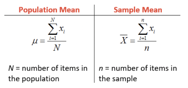
Mean. The mean of a sample or a population is computed by adding all of the observations and dividing by the number of observations.
Example: The Mean of 4,5,6,7 is ( 4+5+6+7 ) / 4 = 5.5
Median. To find the median, we arrange the observations in order from smallest to largest value. If there is an odd number of observations, the median is the middle value. If there is an even number of observations, the median is the average of the two middle values.
Example: The median of 4,1,7 is 4 because when the numbers are put in order ( 1, 4, 7 ) the number 4 is in the middle.
Mode. The most frequent number—that is, the number that occurs the highest number of times.
Example: The mode of { 4, 4, 2, 3, 2, 2} is 2 because it occurs 3 times which is more than any other number.
When to use Median over Mode?
As measures of central tendency, the mean and the median each have advantages and disadvantages. Some pros and cons of each measure are summarised below.
The median may be a better indicator of the most typical value if a set of scores has an outlier. An outlier is an extreme value that differs greatly from other values.
However, when the sample size is large and does not include outliers, the mean score usually provides a better measure of central tendency.
Example: Suppose we examine a sample of 10 households to estimate the typical family income. Nine of the households have incomes between $20,000 and $100,000, but the tenth household has an annual income of $1,000,000,000. That tenth household is an outlier. If we choose a measure to estimate the income of a typical household, the mean will greatly overestimate the income of a typical family (because of the outlier); while the median will not.
Population and Samples
The study of statistics revolves around the study of data sets. There are two important types of data sets
Population. A population includes all of the elements from a set of data.
Samples. A sample consists of one or more observations drawn from the population.
A measurable characteristic of a population, such as a mean or standard deviation, is called a parameter But a measurable characteristic of a sample is called a statistic. We will see in future lessons that the mean of a population is denoted by the symbol μ; but the mean of a sample is denoted by the symbol x̅
Samples are subset’s of population


